Detecting misplaced NG tubes ongoing
• SAFEHR team
A Nasogastric tube (NGT) is a thin tube that is passed into the stomach via the nose for short- to medium-term nutritional support, medication administration or aspiration of stomach contents. NGTs are amongst the most commonly used catheters in critically ill patients in intensive care units (ICU) and high-dependency units and departments where patients require nutritional-support (i.e., Stroke units). Due to increases in the number of hospitalized patients, it is estimated that approximately 10 million NGTs are used annually in Europe, 1 million of which in the UK (~1.2 million in the US).
Previous research highlights a variety of complications associated with NGT placement, which can range from minor cases of nose bleeds to inhalation of stomach contents into the lung and even death. Instances of unknowingly misplaced NGTs being used for feeding, with the feed entering the patients lungs are classified by the NHS as Never Events: “serious incidents that are entirely preventable because guidance or safety recommendations providing strong systemic protective barriers are available at a national level, and should have been implemented by all healthcare providers”.
While all this highlights the importance for feeding tubes in particular to be placed properly and used safely, clinical studies demonstrate that up to 3% of NGTs are reported as misplaced into the airways, causing complications in up to 40% of these cases.
Given the serious complications that can occur from NGT misplacement, UCLH has a detailed policy describing the indications and technique of NGT insertion alongside nationally agreed standards for positioning verification. This includes training and guidelines for doctors or reporting radiographers when checking NGT position radiographically. In this policy, the first line of test in confirming the correct positioning of a feeding tube is by obtaining a sample of fluid from the stomach that shows a level of acidity indicative of the stomach. However, since this cannot be achieved successfully for some patients, and with a large proportion of ICU patients receiving anti-acid medication, the use of CXRs remains the most definitive test for checking NGT placement.
Due to the large number of CXRs obtained each day, especially in intensive and emergency care, and with a limited number of radiologists available, image interpretation can be substantially delayed. Thus, current practices indicate that it is often emergency and ICU doctors who check the CXR to verify the NGT’s correct positioning and suitability for use prior to the radiology report being issued. Yet, such assessments by non-radiologists working in stressful situations when hospitals are capacity, are prone to both human error and some delays in assessment. This means that sub-optimally positioned NGTs can be missed initially, but are often picked up by the radiologists later. This emphasizes the importance of early detection of misplaced NGTs to allow for more timely correction and prevent any additional complications.
We envision two main use scenarios in which an accurate, instant detection and notification of NGT misplacements from CXRs could benefit clinical practice:
(1) As an early alert to ICU doctors or nurses, it will enable prompt, data driven decision-making and NGT adjustment for more effective and safe use. (2) As an early alert to help prioritize the review of most urgent CXRs by local (UCLH) radiologists to reduce delays in notifying ICU doctors of potentially unrecognized NGT misplacement.
Initially, this work focuses on developing a machine learning model to identify misplaced NG tubes on CXR. We will also study ML integration within the ICU at UCLH due to its already established all-digital end-to-end radiology workflow, and to ensure that the sickest, most dependent patients in the hospital will get treatment faster and more safely. In parallel, we will study requirements for future ML system roll outs to any other inpatient area that frequently places NGTs. In a first instance, this will include Stroke Departments within UCLH.
The work can also generate a training opportunity leveraging known cases of misplaced NGTs or cases that were hard to interpret on CXRs. The training datasets can upskill ICU and Stroke ward doctors who often have little experience of assessing such CXRs in routine practice.
Frequency of OMOP concepts in clinical tables
Code
# PROJECT SETUP

# #################### Libraries #################### #
library(here)
library(tidyverse)
library(dbplyr, warn.conflicts = FALSE)
library(rlang, warn.conflicts = FALSE)
library(odbc)


# #################### Constants #################### #
CONFIG_PATH <- "config/db_config.yml"

OMOP_TABLES_DIR <- "res/tables/"
OMOP_COLUMNS_DIR <- "res/columns/"

INPUT_TABLES_FILE <- "clinical.txt"
OUTPUT_PATH <- "out/concept_frequency.csv"


# #################### Functions: Data #################### #

# Higher order function to conditionally apply a pipe
# Note that the cond is not vectorised (should be a single logical)
pipe_if <- function(df, cond, func) {
    if (cond) func(df)
    else df
}

# Load the list of OMOP clinical tables
load_table_list <- function(filename) {
    read_delim(
        file = here(paste0(OMOP_TABLES_DIR, filename)),
        delim = ",",
        col_names = FALSE,
        col_types = "c",
        show_col_types = FALSE)$X1 |>
    map(function(t) { tolower(t) })
}

# Load OMOP column specs for the given table
load_column_metadata <- function(table) {
    read_csv(
        file = here(paste0(OMOP_COLUMNS_DIR, table, "_column_spec.csv")),
        col_types = "cIlcccllcIc",
        show_col_types = FALSE)
}

# Load OMOP column specs extracting Concept columns
load_concept_columns <- function(table) {
    OMOP_VER <- 53
    OMOP_CONCEPT_TYPE <- "concept"

    load_column_metadata(table) |>
    filter(version <= OMOP_VER, type == OMOP_CONCEPT_TYPE) |>
    pull(column)
}

# Debugging output
#
#clinical_tables <- load_table_list("clinical.txt")
#clinical_tables
#
# concepts_by_table <- clinical_tables |>
#     # keep(function(t) { t == "person" || t == "death" }) |>
#     map(function(t) { l <- list(); l[[t]] <- load_concept_columns(t); l }) |>
#     list_flatten()
# concepts_by_table
# map(ls(concepts_by_table), function(t) { list(t, concepts_by_table[[t]] |> as.list()) })


# Load DB configuration
db_load_config <- function(filepath) {
    config = config::get(file = here(filepath))
}

# Connect to a database from the given config
db_connect <- function(config) {
    # Load DB connection
    dbConnect(
        odbc(),
        driver = as.character(config["odbc_driver"]),
        database = as.character(config["odbc_database"]),
        server = as.character(config["odbc_server"]),
        port = as.integer(config["odbc_port"]),
        uid = as.character(config["odbc_uid"]),
        pwd = as.character(config["odbc_pwd"]))
}

# Load table from DB
db_omop_table <- function(tablename, config, conn, cols=NULL) {
    tbl(conn, in_schema(as.character(config["odbc_schema"]), tablename)) |>
    pipe_if(! missing(cols), \(df) df |> select(all_of(cols))) |>
    # head() |>                                               # Head of all tables
    # pipe_if(tablename != "concept", \(df) df |> head()) |>  # Head of non Concept tables
    collect()
}

# Enrich given data frame with the count by column, and include table and column names as metadata
count_with_metadata <- function(df, tablename, colname) {
    df |>
    rename(concept = all_of()) |>
    count(concept, name="count") |>
    mutate(
        table=tablename,
        column=colname,
        .before=concept)
}

# Enrich data frame adding concept names
join_with_concept <- function(df, concepts_df) {
    df |>
    left_join(
        concepts_df,
        by=join_by(concept == concept_id))
}


# #################### Functions: Plots #################### #

# Arranges rows by "count" and update factor levels (for the arrangement to be respected by plots)
arrange_by_count <- function(.df) {
    .df |>
    # Arrange by count, which sorts the dataframe but NOT the factor levels
    arrange(desc(count)) |>
    # Update the factor levels
    mutate(concept_name=fct_reorder(concept_name, count))
}

# Groups rows by concept name, summarising the counts
group_by_name <- function(.df) {
    .df |>
    group_by(concept_name) |>
    summarise(count=sum(count))
}

# Returns a vector of N colours (N <= 12) to use as palette
get_palette <- function(n) {
    c("#009cdb", "#00a3c0", "#00a599", "#33a46f", "#6e9e4c", "#9a933c",
      "#bd8445", "#d57562", "#db6d8a", "#cc72b2", "#a881d3", "#7090e2") |>
    head(n)
}

# Returns a bar plot of frequency counts
freq_bar_plot <- function(.df, head=30, title="", fill="#999999") {
    .df |>
    group_by_name() |>
    arrange_by_count() |>
    head(head) |>
    ggplot(aes(x=concept_name, y=count)) +
        geom_bar(stat="identity", fill=fill, width=.6) +
        coord_flip() +
        xlab("") +
        scale_x_discrete(label=function(x) { stringr::str_trunc(x, 50) }) +
        ggtitle(label=title) +
        theme_bw()
}

# Returns a pie plot of concept distribution with percentages
dist_pie_plot <- function(.df, head=10, title="", fill=c(), border="white") {
    .df |>
    group_by_name() |>
    arrange_by_count() |>
    head(head) |>
    # Calculate count %
    mutate(percent = round(count / sum(.df$count) * 100)) |>
    # Plot
    ggplot(aes(x="", y=count, fill=concept_name)) +
        geom_bar(stat="identity", width=1, colour="white") +
        coord_polar("y", start=0) +
        # Remove background, grid, numeric labels
        theme_void() +
        # Embed count %
        geom_text(
            aes(label=paste0(percent, "%")),
            position=position_stack(vjust=0.5),
            colour="white", fontface = "bold", size=6) +
        # Title and colour
        ggtitle(label=title) +
        scale_fill_manual(values=fill)
}
Data Processing
Frequency table
Frequency table for OMOP concepts in clinical tables.
Clincial tables are:
- CARE_SITE
- CONDITION_OCCURRENCE
- DEATH
- DEVICE_EXPOSURE
- DRUG_EXPOSURE
- FACT_RELATIONSHIP
- LOCATION
- MEASUREMENT
- OBSERVATION_PERIOD
- OBSERVATION
- PERSON
- PROCEDURE_OCCURRENCE
- SPECIMEN
- VISIT_DETAIL
- VISIT_OCCURRENCE
Code
# DATA PROCESSING

# Generate frequency table for OMOP concepts in clinical tables

db_config <- db_load_config(CONFIG_PATH)
db_conn = db_connect(db_config)

start_time <- Sys.time()

# Load all Concepts to find names
concepts_df <- db_omop_table("concept", db_config, db_conn, cols=c("concept_id", "concept_name"))

concept_freq <- tibble()
for (tablename in load_table_list(INPUT_TABLES_FILE)) {
    # Table from DB
    df <- db_omop_table(tablename, db_config, db_conn)

    # Add to metadata
    for (colname in load_concept_columns(tablename)) {
        #message("count_with_metadata: Processing ", tablename, ".", colname)
        concept_freq <- bind_rows(
           concept_freq,
           count_with_metadata(df, tablename, colname))
    }
}

concept_freq <- concept_freq |>

# Remove lines with count < 5
filter(count >= 5) |>

# Sort by concept
arrange(table, column, concept) |>

# Join with Concept to include names
join_with_concept(concepts_df)

# Calculate processing time
end_time <- Sys.time()
message("Generated in ", sprintf("%.2f", as.numeric(end_time - start_time, units="mins")), " minutes")

# Export and print result
concept_freq |> write_csv(OUTPUT_PATH)
concept_freq


# [WIP] Attempts to generate frequency table with functional programming
#
# load_table_list("clinical.txt") |>
# # keep(function(t) { t == "person" || t == "death" }) |>
# map(function(t) {
#     load_concept_columns(t) |>
#     map(function(c) {
#         count_with_metadata(
#             db_omop_table(schema, t, conn=conn),
#             t, c)
#     })
# }) |>
# bind_rows()

dbDisconnect(db_conn)| table | column | concept | count | concept_name |
|---|---|---|---|---|
| <chr> | <chr> | <int> | <int> | <chr> |
| care_site | place_of_service_concept_id | 8717 | 23 | Inpatient Hospital |
| condition_occurrence | condition_concept_id | 22274 | 33 | Neoplasm of uncertain behavior of larynx |
| condition_occurrence | condition_concept_id | 22281 | 212 | Sickle cell-hemoglobin SS disease |
| condition_occurrence | condition_concept_id | 22350 | 5 | Edema of larynx |
| condition_occurrence | condition_concept_id | 22492 | 5 | Foreign body in pharynx |
| condition_occurrence | condition_concept_id | 22557 | 13 | Malignant tumor of submandibular gland |
| condition_occurrence | condition_concept_id | 22955 | 28 | Perforation of esophagus |
| condition_occurrence | condition_concept_id | 23034 | 153 | Neonatal hypoglycemia |
| condition_occurrence | condition_concept_id | 23220 | 28 | Chronic tonsillitis |
| condition_occurrence | condition_concept_id | 23325 | 58 | Heartburn |
| condition_occurrence | condition_concept_id | 23986 | 39 | Disorder of pituitary gland |
| condition_occurrence | condition_concept_id | 24006 | 42 | Sickle cell-hemoglobin C disease |
| condition_occurrence | condition_concept_id | 24134 | 150 | Neck pain |
| condition_occurrence | condition_concept_id | 24148 | 33 | Congenital diverticulum of pharynx |
| condition_occurrence | condition_concept_id | 24609 | 226 | Hypoglycemia |
| condition_occurrence | condition_concept_id | 24660 | 28 | Acute tonsillitis |
| condition_occurrence | condition_concept_id | 24818 | 7 | Injury of neck |
| condition_occurrence | condition_concept_id | 24909 | 17 | Hereditary spherocytosis |
| condition_occurrence | condition_concept_id | 24966 | 49 | Esophageal varices |
| condition_occurrence | condition_concept_id | 24974 | 5 | Stenosis of larynx |
| condition_occurrence | condition_concept_id | 25189 | 27 | Malignant tumor of oral cavity |
| condition_occurrence | condition_concept_id | 25518 | 231 | Sickle cell trait |
| condition_occurrence | condition_concept_id | 25572 | 5 | Disorder of salivary gland |
| condition_occurrence | condition_concept_id | 25582 | 24 | Tracheoesophageal fistula |
| condition_occurrence | condition_concept_id | 25844 | 8 | Ulcer of esophagus |
| condition_occurrence | condition_concept_id | 26052 | 28 | Primary malignant neoplasm of larynx |
| condition_occurrence | condition_concept_id | 26141 | 5 | Barrett's esophagus with esophagitis |
| condition_occurrence | condition_concept_id | 26727 | 46 | Hematemesis |
| condition_occurrence | condition_concept_id | 26942 | 83 | Hemoglobin SS disease with crisis |
| condition_occurrence | condition_concept_id | 27674 | 183 | Nausea and vomiting |
| ⋮ | ⋮ | ⋮ | ⋮ | ⋮ |
| specimen | specimen_concept_id | 40490358 | 21 | Specimen from skin obtained by scraping |
| specimen | specimen_concept_id | 40490923 | 10 | Foreign body submitted as specimen |
| specimen | specimen_concept_id | 40490924 | 11 | Urine specimen from urinary conduit |
| specimen | specimen_concept_id | 43021080 | 5 | Swab from lower limb |
| specimen | specimen_concept_id | 43021097 | 12 | Swab from pharynx |
| specimen | specimen_concept_id | 43021144 | 14 | Central venous catheter tip submitted as specimen |
| specimen | specimen_concept_id | 43021146 | 22 | Arterial line tip submitted as specimen |
| specimen | specimen_concept_id | 44783230 | 14 | Urine specimen obtained via suprapubic indwelling urinary catheter |
| specimen | specimen_concept_id | 44784239 | 22 | First stream urine sample |
| specimen | specimen_concept_id | 45766301 | 16 | Arterial cord blood specimen |
| specimen | specimen_concept_id | 45766302 | 13 | Venous cord blood specimen |
| specimen | specimen_concept_id | 46270252 | 69 | Specimen from bronchus obtained by endobronchial biopsy |
| specimen | specimen_concept_id | 46273457 | 5 | Brain cyst fluid sample |
| specimen | specimen_type_concept_id | 32817 | 182136 | EHR |
| specimen | unit_concept_id | 0 | 182136 | No matching concept |
| visit_occurrence | admitting_source_concept_id | 0 | 9795 | No matching concept |
| visit_occurrence | admitting_source_concept_id | 8602 | 26 | Temporary Lodging |
| visit_occurrence | admitting_source_concept_id | 8717 | 94 | Inpatient Hospital |
| visit_occurrence | discharge_to_concept_id | 0 | 164 | No matching concept |
| visit_occurrence | discharge_to_concept_id | 8536 | 9543 | Home |
| visit_occurrence | discharge_to_concept_id | 8602 | 37 | Temporary Lodging |
| visit_occurrence | discharge_to_concept_id | 8615 | 16 | Assisted Living Facility |
| visit_occurrence | discharge_to_concept_id | 8717 | 128 | Inpatient Hospital |
| visit_occurrence | discharge_to_concept_id | 8882 | 14 | Adult Living Care Facility |
| visit_occurrence | discharge_to_concept_id | 8971 | 12 | Inpatient Psychiatric Facility |
| visit_occurrence | visit_concept_id | 262 | 918 | Emergency Room and Inpatient Visit |
| visit_occurrence | visit_concept_id | 9201 | 5525 | Inpatient Visit |
| visit_occurrence | visit_concept_id | 9203 | 3472 | Emergency Room Visit |
| visit_occurrence | visit_source_concept_id | NA | 9915 | NA |
| visit_occurrence | visit_type_concept_id | 32817 | 9915 | EHR |
Figures
The plots below are based on the frequencies of concepts in clinical tables.
Null values and the following special concepts have been ignored: - 0: Used when there is no matching concept between the source value and the standard defined by OMOP. - 32817: EHR, indicating that the source of the information is the EHR system.
Code
# FIGURES

# General options
options(repr.plot.width=12)

# Load data (or reuse data frame)
#plot_df_all <- concept_freq
plot_df_all <- read_csv(file = here(OUTPUT_PATH), col_types = "cciic")

# Ignore null, 0, and EHR (32817)
plot_df <- plot_df_all |>
filter(concept > 0) |>    # Ignore nulls and No matching concept
filter(concept != 32817)  # Ignore concept "EHR"
Top concepts
See Figure 1 for concepts appearing the most often in all clinical tables.
Since the table measurement contains a much larger number of records than other clinical tables, the concepts with the higher frequency mostly come from it.
Top measurements
See Figure 2 for the measurements recorded the most often.
This information is taken from table measurement, column measurement_concept_id.
Top conditions
See Figure 3 for the most frequent conditions.
This information is taken from table condition_occurrence, column condition_concept_id.
Gender distribution
See Figure 4 to understand the distribution of gender in all patients.
Procedures
See Figure 5 to understand the distribution of procedures performed.
This information is taken from from table procedure_occurrence, column procedure_concept_id.
Visits
See Figure 6 to understand the distribution of visits received.
This information is taken from from table visit_occurrence, column visit_concept_id.
Example (synthetic) Electronic Health Record data
These data are modelled using the OMOP Common Data Model v5.3.
CSV files
The name of the file corresponds to the table in the OMOP CDM.
Correlated Data Source
- NG tube vocabularies
Generation Rules
- The patient’s age should be between 18 and 100 at the moment of the visit.
- Ethnicity data is using 2021 census data in England and Wales (Census in England and Wales 2021) .
- Gender is equally distributed between Male and Female (50% each).
- Every person in the record has a link in procedure_occurrence with the concept “Checking the position of nasogastric tube using X-ray”
- 2% of person records have a link in procedure_occurrence with the concept of “Plain chest X-ray”
- 60% of visit_occurrence has visit concept “Inpatient Visit”, while 40% have “Emergency Room Visit”
Notes
- Version 0
- Generated by man-made rule/story generator
- Structural correct, all tables linked with the relationship
- We used national ethnicity data to generate a realistic distribution (see below)
2011 Race Census figure in England and Wales
| Ethnic Group | Population(%) |
|---|---|
| Asian or Asian British: Bangladeshi | 1.1 |
| Asian or Asian British: Chinese | 0.7 |
| Asian or Asian British: Indian | 3.1 |
| Asian or Asian British: Pakistani | 2.7 |
| Asian or Asian British: any other Asian background | 1.6 |
| Black or African or Caribbean or Black British: African | 2.5 |
| Black or African or Caribbean or Black British: Caribbean | 1 |
| Black or African or Caribbean or Black British: other Black or African or Caribbean background | 0.5 |
| Mixed multiple ethnic groups: White and Asian | 0.8 |
| Mixed multiple ethnic groups: White and Black African | 0.4 |
| Mixed multiple ethnic groups: White and Black Caribbean | 0.9 |
| Mixed multiple ethnic groups: any other Mixed or multiple ethnic background | 0.8 |
| White: English or Welsh or Scottish or Northern Irish or British | 74.4 |
| White: Irish | 0.9 |
| White: Gypsy or Irish Traveller | 0.1 |
| White: any other White background | 6.4 |
| Other ethnic group: any other ethnic group | 1.6 |
| Other ethnic group: Arab | 0.6 |
Example (synthetic) images
Model
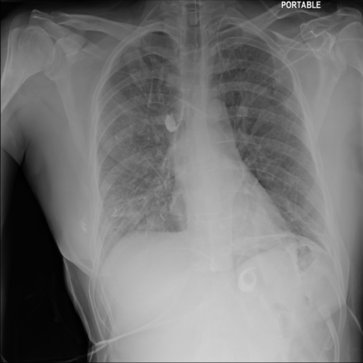
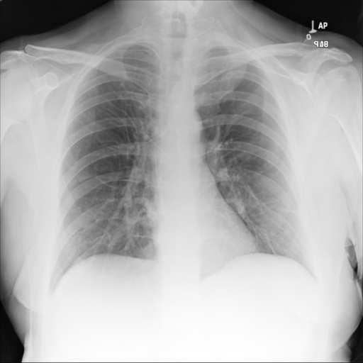
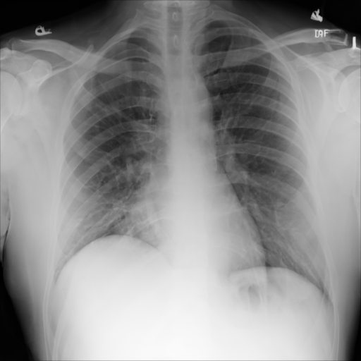
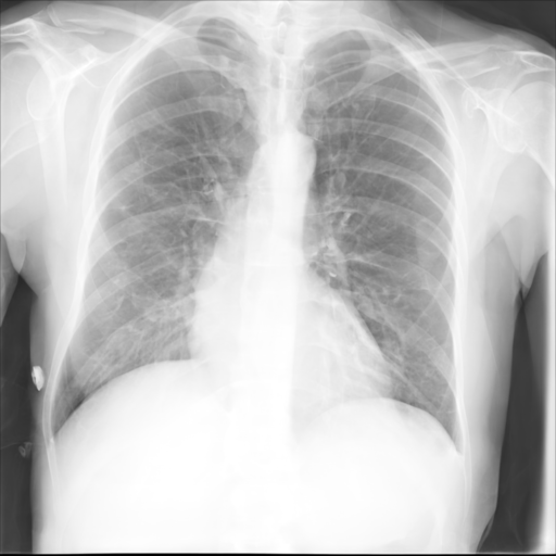
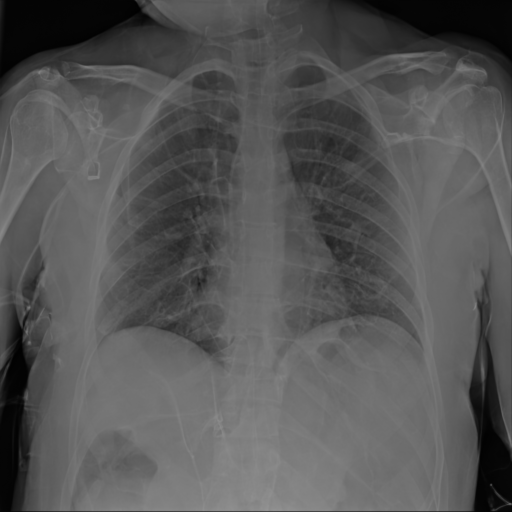
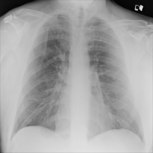
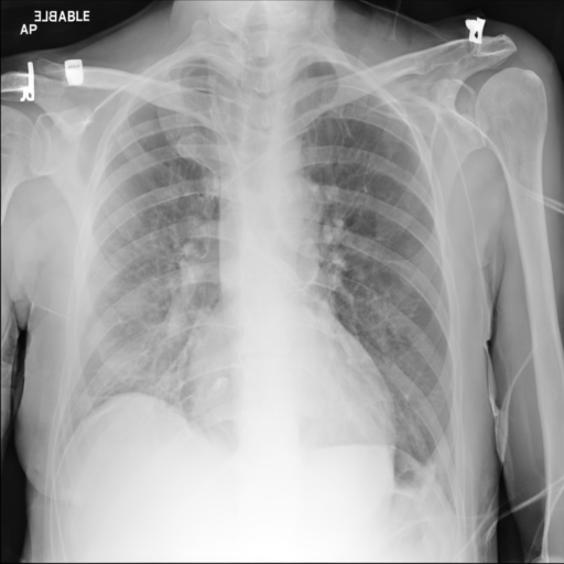
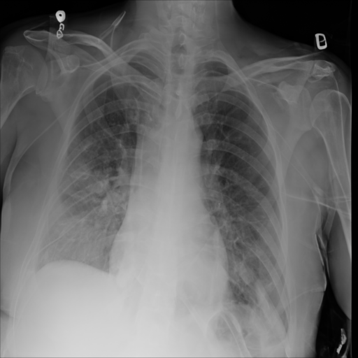
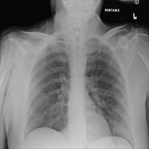
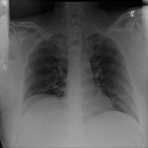
A Hugging Face Unconditional image generation Diffusion Model was used for training. [1] Unconditional image generation models are not conditioned on text or images during training. They only generate images that resemble the training data distribution. The model usually starts with a seed that generates a random noise vector. The model will then use this vector to create an output image similar to the images used to train the model. The training script initializes a UNet2DModel and uses it to train the model. [2] The training loop adds noise to the images, predicts the noise residual, calculates the loss, saves checkpoints at specified steps, and saves the generated models.
Training Dataset
The RANZCR CLiP dataset was used to train the model. [3] This dataset has been created by The Royal Australian and New Zealand College of Radiologists (RANZCR) which is a not-for-profit professional organisation for clinical radiologists and radiation oncologists. The dataset has been labelled with a set of definitions to ensure consistency with labelling. The normal category includes lines that were appropriately positioned and did not require repositioning. The borderline category includes lines that would ideally require some repositioning but would in most cases still function adequately in their current position. The abnormal category included lines that required immediate repositioning. 30000 images were used during training. All training images were 512x512 in size. Computational Information Training has been conducted using RTX 6000 cards with 24GB of graphics memory. A checkpoint was created after each epoch was saved with 220 checkpoints being generated so far. Each checkpoint takes up 1GB space in memory. Generating each epoch takes around 6 hours. Machine learning libraries such as TensorFlow, PyTorch, or scikit-learn are used to run the training, along with additional libraries for data preprocessing, visualization, or deployment.
References
- https://huggingface.co/docs/diffusers/en/training/unconditional_training#unconditional-image-generation
- https://github.com/huggingface/diffusers/blob/096f84b05f9514fae9f185cbec0a4d38fbad9919/examples/unconditional_image_generation/train_unconditional.py#L356
- https://www.kaggle.com/competitions/ranzcr-clip-catheter-line-classification/data